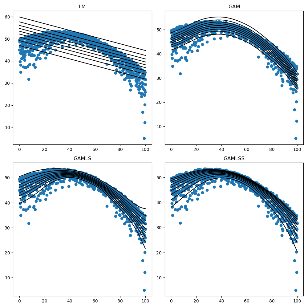
From LM to GAMLSS

This script demonstrates the progression from Linear Model (LM) to Generalized Additive Models for Location, Scale, and Shape (GAMLSS) using the sknormod package.

Imports

import numpy as np
import matplotlib.pyplot as plt

from sknormod import gam
from sknormod import NormodOLS

from sknormod.datasets import make_lss_SHASHo2
from sknormod.plotting import plot_scatter_with_lines

Ploting functions

Define a custom plotting function to visualize the models

def plot_model(ax, x, y, normod, title):
    # Generate centiles for prediction
    centiles = np.linspace(0.1, 0.9, 9)
    # Predict centiles using the normative model
    predicted_centiles = normod.predict_distr_p(x, centiles)
    # Plot scatter plot of data points
    ax.scatter(x, y)
    # Plot centile lines
    for centile_line in predicted_centiles:
        ax.plot(x, centile_line, color='black')
    # Set title for the subplot
    ax.set_title(title)

Simulate data

Generate synthetic data for demonstration

x, y = make_lss_SHASHo2(1000,
                        interpolate_mu=[50, 52, 35],
                        interpolate_sigma=[2, 0.5, 2],
                        interpolate_nu=[-1.5, -1.5],
                        interpolate_tau=[1, 1])
# Reshape the feature array to match the model input requirements
x = x.reshape(-1, 1)

Fit models

Initialize normative models: OLS, GAM, GAMLS, and GAMLSS

normod_ols = NormodOLS()  # Linear Model
normod_gam = gam.GAM(mu_formula="y ~ s(x0)")  # GAM
normod_gam_ls = gam.GAMLS(mu_formula="y ~ s(x0)",
                        sigma_formula=" ~ s(x0)")  # GAM Heteroskedastic (LS)
normod_gam_lss = gam.GAMLSS(mu_formula="y ~ s(x0)",
                            sigma_formula=" ~ s(x0)",
                            nu_formula=" ~ 1",
                            tau_formula=" ~ 1")  # GAMLSS

# Fit the models to the data
normod_ols.fit(x, y)
normod_gam.fit(x, y)
normod_gam_ls.fit(x, y)
normod_gam_lss.fit(x, y)

GAMLSS(mu_formula='y ~ s(x0)', nu_formula=' ~ 1', sigma_formula=' ~ s(x0)',
       tau_formula=' ~ 1')

In a Jupyter environment, please rerun this cell to show the HTML representation or trust the notebook.
On GitHub, the HTML representation is unable to render, please try loading this page with nbviewer.org.

Visualize the results

estimated_centiles = list((
    normod.predict_distr_p(x, np.linspace(0.1, 0.9, 9))
    for normod in [normod_ols, normod_gam, normod_gam_ls, normod_gam_lss]
))

fig, axes = plt.subplots(2, 2, figsize=(10, 10))
titles = ["LM", "GAM", "GAMLS", "GAMLSS"]
for i_col, ax in enumerate(axes.flat):
    plt.sca(ax)
    plot_scatter_with_lines(x, y, lines=estimated_centiles[i_col], cbar=False)
    ax.set_title(titles[i_col])
plt.tight_layout()
plt.show()

/home/brick/Code/scikit-normod/sknormod/plotting.py:6: UserWarning: No data for colormapping provided via 'c'. Parameters 'cmap' will be ignored
  plt.scatter(x, y, c=c, cmap="coolwarm")