Plotting NormodOLS normative model

This example showcases the usage of the NormodOLS class from the sknormod library. It focuses on fitting a normative model using ordinary least squares (OLS) regression, followed by visualizing the results including centiles and z-scores.

Import necessary libraries

import numpy as np
from sknormod import NormodOLS
from sknormod.plotting import plot_scatter_with_lines
from sknormod.datasets import make_gaussian

Simulate Data

Generate synthetic data mimicking a population’s age-related variable (e.g., cognitive score) and their corresponding age. Here, we create a sample of 500 individuals.

n_subj = 500
age, y = make_gaussian(n_subj, interpolate_mu=[95, 98, 92])
# We also generate a quadratic feature of age to capture potential nonlinear
# relationships.
X = np.column_stack((age, age**2))

Fitting Normative Model

We employ the NormodOLS class, which implements Ordinary Least Squares (OLS) regression for normative modeling.

normod = NormodOLS()
# Fit the normative model using the generated data.
normod.fit(X, y)

NormodOLS()

In a Jupyter environment, please rerun this cell to show the HTML representation or trust the notebook.
On GitHub, the HTML representation is unable to render, please try loading this page with nbviewer.org.

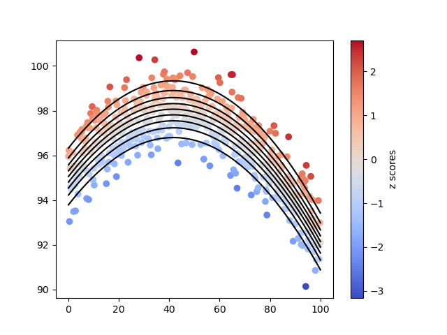
Get centiles and z-scores

Generating Centiles and Z-Scores Once the model is fitted, we can use it to predict centiles and calculate z-scores for new observations. We predict centiles at specific percentiles (e.g., 10th, 20th, …, 90th).

# Now the centiles
estimated_centiles = normod.predict_distr_p(X, np.linspace(0.1, 0.9, 9))
# We also transform the observed data into z-scores.
subjects_z_scores = normod.transform_to_z(X, y)

Plotting Results

Finally, we visualize the fitted model along with the centiles and the distribution of z-scores.

plot_scatter_with_lines(age, y, lines=estimated_centiles, c=subjects_z_scores)

<module 'matplotlib.pyplot' from '/home/brick/miniconda3/lib/python3.12/site-packages/matplotlib/pyplot.py'>