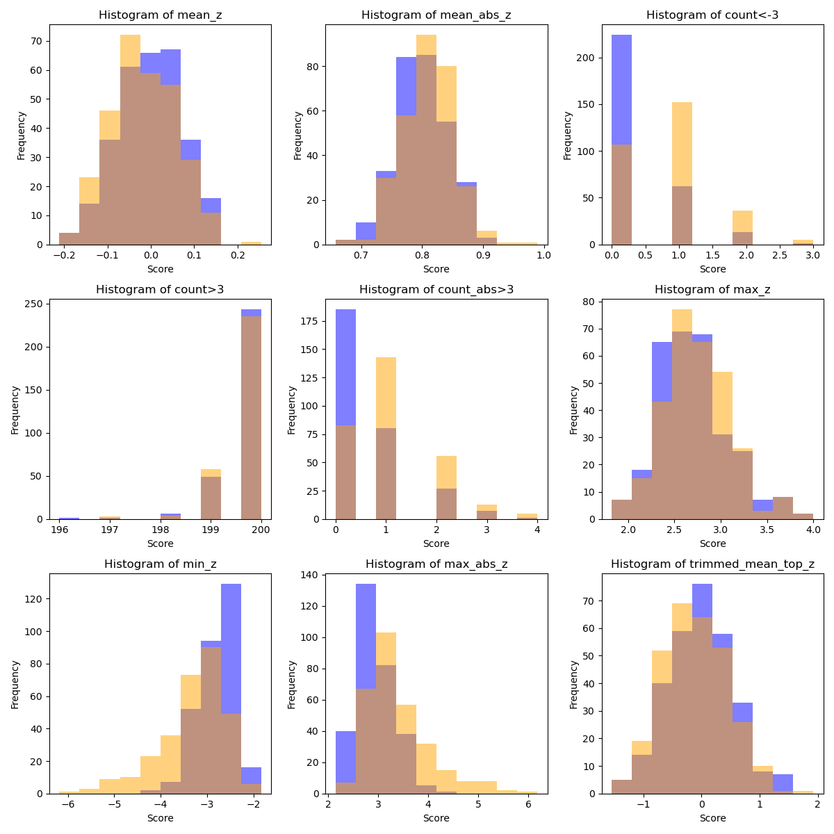
Anomaly scores

calculating anomaly scores

import numpy as np
import matplotlib.pyplot as plt
from sknormod import MassUnivNormodOLS
from sknormod.datasets import make_gaussian
from sknormod.plotting import plot_scatter_with_lines
from sknormod.atypicality import multi_atypicality_scorer, multi_roc_auc_score

from sklearn.model_selection import train_test_split

Generate synthetic data

We generate synthetic data for multiple variables across a range of ages.

n_subj = 2000  # Number of subjects
n_cols = 200    # Number of variables

age = np.linspace(0, 100, n_subj)
X = np.column_stack((age, age**2))  # Age and age squared as features
# Generate synthetic Y data for each variable
Y = np.column_stack([make_gaussian(n_subj,
        interpolate_mu = np.random.normal(loc=100, scale=2, size=3))[1]
                     for _ in range(n_cols)])

train test split and generate test data

X_train, X_test, Y_train, Y_test = train_test_split(X, Y, test_size=0.3)

n_test = X_test.shape[0]
diag_labels = np.array([0]*(n_test//2) + [1]*(n_test//2))

num_cols = 50
rows_to_modify = np.where(diag_labels == 1)[0]

# For each row that meets the condition, subtract 0.1 from a random column
for row in rows_to_modify:
    # Randomly select a column index
    col_index = np.random.choice(num_cols)
    # Subtract 0.1 from the selected column in the current row
    Y_test[row, col_index] -= 3

Fit and get z-scores and abnormality scores

# Fit MassUnivNormodOLS model
mass_normod = MassUnivNormodOLS()
mass_normod.fit(X_train, Y_train)

# Calculate z-scores
Z_test = mass_normod.transform_to_z(X_test, Y_test)
# Calculate abnormality scores
atypicality_scores = multi_atypicality_scorer(Z_test)

# Check how well they discirminate between groups
auc_scores = multi_roc_auc_score(diag_labels, atypicality_scores)
for key, value, in auc_scores.items():
    print(f"{key}: {value:.2f}")

mean_z: 0.56
mean_abs_z: 0.57
count<-3: 0.70
count>3: 0.51
count_abs>3: 0.68
max_z: 0.54
min_z: 0.74
max_abs_z: 0.72
trimmed_mean_top_z: 0.55

Ploting

n_columns = len(atypicality_scores)
# Number of rows and columns for subplots
n_rows = (n_columns + 2) // 3
n_cols = min(n_columns, 3)

# Create a figure with subplots (3 columns)
fig, axes = plt.subplots(n_rows, n_cols, figsize=(12, 4 * n_rows), tight_layout=True)
# Flatten the axes array
axes = axes.flatten()
# Plot a histogram for each score type in the dictionary
for i, (score_name, scores) in enumerate(atypicality_scores.items()):
    ax = axes[i]
    min_value = np.min(scores)
    max_value = np.max(scores)
    ax.hist(scores[diag_labels == 0], range=(min_value, max_value),
            color="blue", alpha=0.5, label='Label 0')
    ax.hist(scores[diag_labels == 1], range=(min_value, max_value),
            color="orange", alpha=0.5, label='Label 1')
    ax.set_title(f'Histogram of {score_name}')
    ax.set_xlabel('Score')
    ax.set_ylabel('Frequency')

# Hide empty subplots if there are fewer scores than subplots
for ax in axes[n_columns:]:
    ax.axis('off')

# Show the plot
plt.show()